[Read Paper] Eyeriss v2: A Flexible and High-Performance Accelerator for Emerging Deep Neural Networks
Published:
by
SingularityKChen
![]() (Last updated:
)
(Last updated:
)
- Categories:
- ReadPaper 30
- Tags:
- DLA 19
- DNN 12
- EyerissV2 2
- Eyexam 1
- Eyeriss v2: A Flexible and High-Performance Accelerator for Emerging Deep Neural Networks
Eyeriss v2: A Flexible and High-Performance Accelerator for Emerging Deep Neural Networks
This article describes:
- a performance analysis framework named
Eyexamwhich provides a seven-step process to systematically identify the source of performance loss and can be used to develop a set ofroofline modelsto quantitatively identify the source of performance loss in DNN processors; - a DNN accelerator named
Eyeriss v2which uses a hierarchicalNoCthat allows the system to exploit spatial data reuse for large DNNs and deliver high bandwidth for compact DNNs with the scalability;
Changes in Performance and Flexibility
Two Bad Ways in Widely Varying Data Reuse
- depend on data reuse in certain data dimensions
- the spatial accumulation array architecture relies on both output and input channels;
- the temporal accumulation array architecture relies on another set of data dimensions;
- the spatial accumulation array architecture relies on both output and input channels;
- lower data reuse need a higher data bandwidth
To Build a Truly Flexible DNN Processor
- the dataflow relies on certain data dimensions for data reuse
- low utilization of the parallelism when those data dimensions diminish
- the NoC and its corresponding memory hierarchy
- high bandwidth and low spatial data reuse;
- low bandwidth and high spatial data reuse scenarios;
- instead of being adaptive to the specific condition of the workload;
- high bandwidth and low spatial data reuse;
Eyexam
Two Main Factors that Affect Performance
- the number of active PEs due to the mapping determined by the dataflow;
- the utilization of active PEs based on whether the NoC has sufficient bandwidth to deliver data to PEs to keep them active;
This is a example dataflow for a 1D CONV:
#include <stdio.h>

int main()
{
 int R2, R1, R0, E2, E1, E0;
 // R0, R1, R2 related to filter
 R2 = 2;//chnl of filter, C, sum of one chnl ofmap
 R1 = 3;//height of filter, R, psum of one row ofmap
 R0 = 4;//width of filter, S, ppsum of one ofmap
 // E0, E1, E2 related to ofmap
 E2 = 2;//chnl of ofmap or number of filters, M, sums in different chnl ofmaps
 E1 = 4;//height of ofmap, E, psum of one chnl ofmap
 E0 = 5;//width of ofmap, F, ppsum of one row ofmap
 int inx_o, inx_i, inx_w;
 for (int e2 = 0; e2 < E2; e2++) {
  for (int r2 = 0; r2 < R2; r2++) {
   for (int e1 = 0; e1 < E1; e1++) {
    for (int r1 = 0; r1 < R1; r1++) {
     for (int e0 = 0; e0 < E0; e0++) {
      for (int r0 = 0; r0 < R0; r0++) {
       inx_o = e2*E1*E0+e1*E0+e0;
       inx_i = e2*E1*E0+e1*E0+e0 + r2*R1*R0+r1*R0+r0;
       inx_w = r2*R1*R0+r1*R0+r0;
       printf("O[%d] += I[%d] * W[%d]\t", inx_o, inx_i, inx_w);
       //printf("O[e2*E1*E0+e1*E0+e0] = O[%d*E1*E0+%d*E0+%d]\n", e2, e1, e0);
       /* code */
      }
      /* code */
      //printf("----------- r0 for loop finished -----------\n");
      printf("\n");
     }
     /* code */
     printf("*********** e0 for loop finished ***********\n");
    }
    /* code */
    printf("+++++++++++ r1 for loop finished +++++++++++\n");
   }
   /* code */
   printf("=========== e1 for loop finished ===========\n");
  }
  /* code */
  printf("@@@@@@@@@@@ r2 for loop finished @@@@@@@@@@@\n");
 }
 return 0;
}
- inner two
forloops represent the temporal processing andSPadaccesses within aPE; - the outer two
forloops represent the temporal processing of multiple passes across thePEarray and GLB accesses; - the two
parallel-fors represent the distribution of computation across multiplePEs;
Seven steps to analyse the performance of an architecture
- layer shape and size: the number of
MACs in the layer - dataflow: the maximum parallelism of the dataflow
- number of
PEs: the theoretical peak performance. Two shape fragmentation:- spatial mapping fragmentation:
RorR1is smaller than the number ofPEs => some are completely idle- temporal mapping fragmentation:
Ris not an integer multiple ofPEs => some are not always active
- temporal mapping fragmentation:
- spatial mapping fragmentation:
- physical dimensions of the
PEarray: the run-time utilization ofPEs due to shape fragmentation for each dimension - storage capacity: reduce the number of active
PEs due to storage of intermediate data. e.g., limited storage forpsums => the limited number of weights be processed in parallel => limited number of activePEs that can operate in parallel - data bandwidth: insufficient average bandwidth to active
PEs. The performance will be bandwidth-limited when the operational intensity is lower than the inflection point - varying data access patterns: insufficient instant bandwidth to active
PEs
Performance Analysis Results for DNN Processors and Workloads
- simply increasing hardware resources is not sufficient to achieve a higher performance
- the dataflow has to be flexible enough to deal the diminished reuse available in any data dimensions
- the NoC design should meet the worst-case bandwidth requirement for every data type
- the NoC design should aim to exploit data reuse to minimize the number of GLB accesses
Flexible Dataflow
The new dataflow named Row-Stationary Plus supports data tiling from all dimensions to fully utilize the PE array.
- additional loops
g1andn1are added at the NoC level to provide more options to parallelize different dimensions of data - allow data to be tiled from multiple dimensions and mapped in parallel onto the same
PEarray dimension - the data tile from the same dimension can also be mapped spatially onto different physical dimensions to fully utilize the
PEarray - allow tile in data dimension
Rwith loopr1 - an additional loop
e0is added at theSPadlevel to create more reuse of weights in theSPad.
inx_o = g3*G2*G1 + g2*G1 + g1
    + n3*N2*N1*N0 + n2*N1*N0 + n1*N0 + n0
    + m3*M2*M1*M0 + m2*M1*M0 + m1*M0 + m0
    + e0
    + f3*F2*F1*F0 + f2*F1*F0 + f1*F0 + f0;
inx_i = g3*G2*G1 + g2*G1 + g1
    + n3*N2*N1*N0 + n2*N1*N0 + n1*N0 + n0
    + e0
    + f3*F2*F1*F0 + f2*F1*F0 + f1*F0 + f0
    + c2*C1*C0 + c1*C0 + c0
    + r0
    + s2*S1 + s1;
inx_w = g3*G2*G1 + g2*G1 + g1
    + m3*M2*M1*M0 + m2*M1*M0 + m1*M0 + m0
    + c2*C1*C0 + c1*C0 + c0
    + r0
    + s2*S1 + s1;

inx_o[0] = m0 + e0*M0 + n0*E0*M0 + f0*N0*E0*M0;
inx_w[0] = m0 + c0*M0 + r0*C0*M0;
inx_i[0] = c0 + r0*C0 + e0*R0*C0 + n0*E0*R0*C0 + f0*N0*E0*R0*C0;
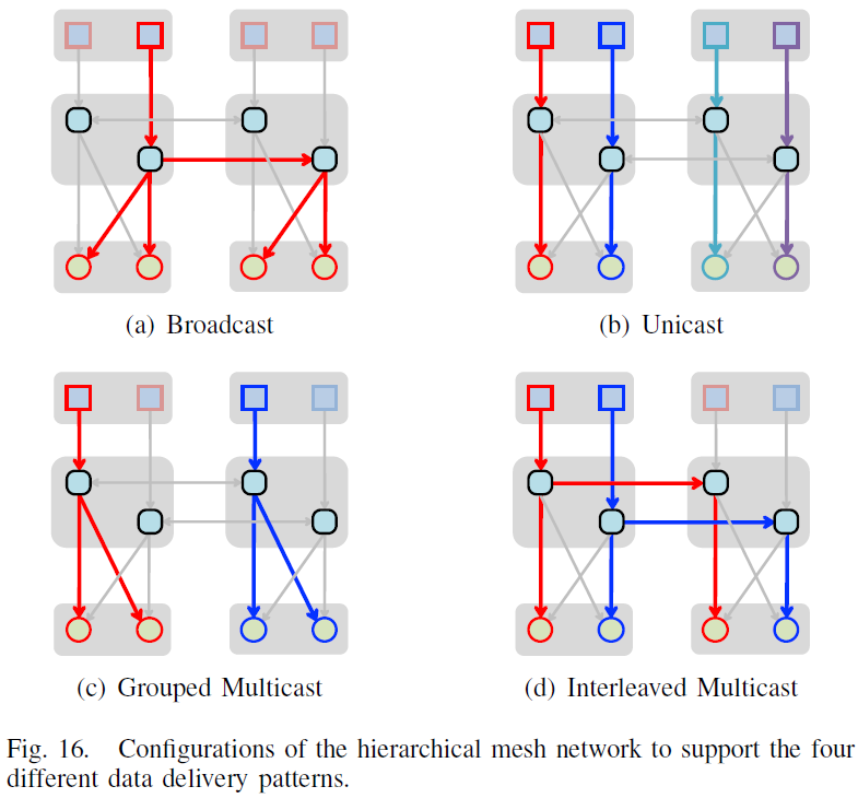
Flexible and Scalable NoC
A new NoC named hierarchical mesh is designed to adapt to a wide range of bandwidth requirements.
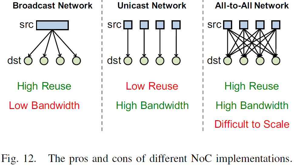
The Pros and Cons of Different NoC Implementations
- Broadcast Network: high reuse but low bandwidth
- Unicast Network: high bandwidth but low reuse
- All-to-All Network: implementation cost and energy consumption increase quadratically
Architecture and Work Models of Hierarchical Mesh Network
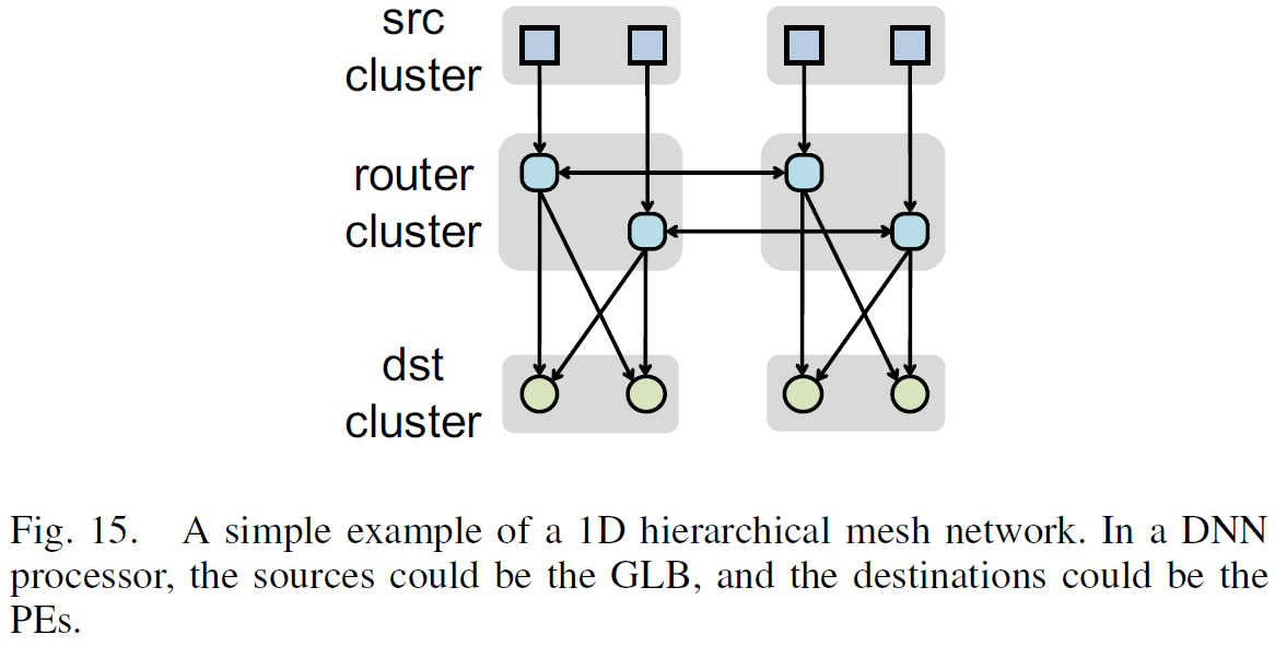
Considerations
The size of clusters:
- what is the bandwidth required from the source cluster in the worst case, i.e., unicast mode;
- what is the bandwidth required in between the router clusters in the worst case, i.e., interleaved multicast mode;
- what is the tolerable cost of the all-to-all network;
The tile size of the mapped data dimensions:
- the cluster size
- the number of clusters