[Glean] Grouped Convolution

Published: May 27, 2021 by SingularityKChen (Last updated: May 27, 2021 )

• Categories:
• Glean 53

• Tags:
• DNN 12
• Grouped Convolution 1
• ML 3

• Grouped Convolution
  • AlexNet
  • Problems that Grouped Convolution solved
  • Convolution vs Grouped Convolution
• Reference

Grouped Convolution

Usually, convolution filters are applied on an image layer by layer to get the final output feature maps.

But to learn more no. of features, we could also create two or more models that train and back propagate in parallel. This process of using different set of convolution filter groups on same image is called as grouped convolution¹ or Filter Groups².

AlexNet²

Filter groups (AKA grouped convolution) were introduced in AlexNet paper in 2012. As explained by the authors, their primary motivation was to allow the training of the network over two Nvidia GTX 580 gpus with 1.5GB of memory each. With the model requiring just under 3GB of GPU RAM to train, filter groups allowed more efficient model-parellization across the GPUs, as shown in the illustration of the network from the paper:

Problems that Grouped Convolution solved¹

By using grouped convolution:

• With grouped convolutions, we can build networks as wide as we want. Take one modular block of filter group and replicate them.
• Now, each filter convolves only on some of the feature maps obtained from kernel filters in its filter group, we are drastically reducing the no of computations to get output feature maps. Of course, you can argue that we are replicating the filter group, resulting in more number of computations. But to keep things in perspective, if we were to take all kernel filters in grouped convolutions and not use the concept of grouped convolutions, the number of computations will grow exponentially.
• We can parallelize the training in two ways:
  • Data parallelism: where we split the dataset into chunks and then we train on each chunk. Intuitively, each chunk can be understood as a mini batch used in mini batch gradient descent. Smaller the chunks, more data parallelism we can squeeze out of it. However, smaller chunks also mean that we are doing more like stochastic than batch gradient descent for training. This would result in slower and sometimes poorer convergence.
  • Model parallelism: here we try to parallelize the model such that we can take in as much as data as possible. Grouped convolutions enable efficient model parallelism, so much so that Alexnet was trained on GPUs with only 3GB RAM.

Apart from solving the above problems, grouped convolutions seem to be learning better representations of the data. Essentially, the correlation between kernel filters of different filter groups is usually quite less, which implies that, each filter group is learning a unique representation of the data.

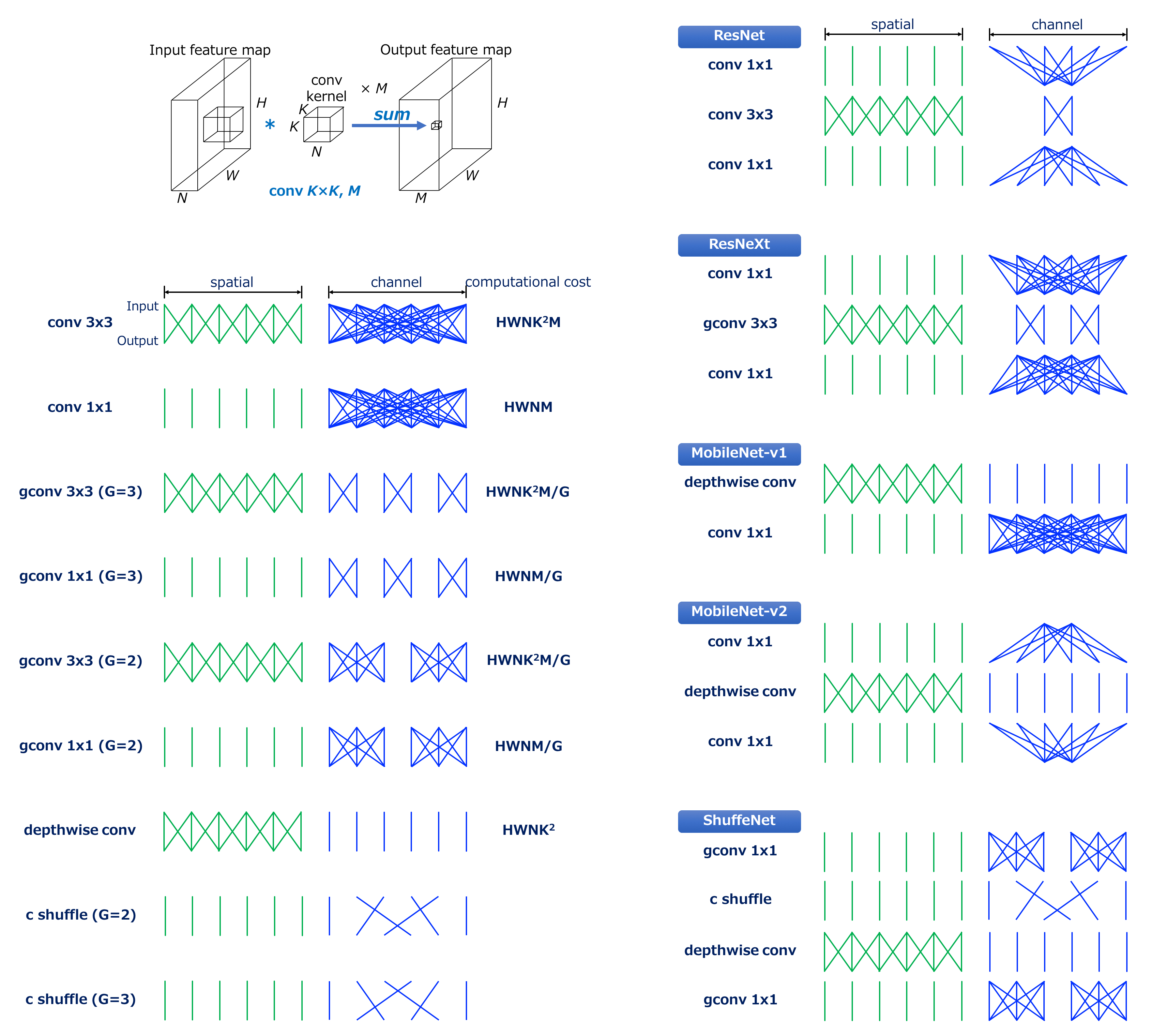
Convolution vs Grouped Convolution³

The number of lines roughly indicate the computational cost of convolution in spatial and channel domain respectively.

For instance, conv3x3, the most commonly used convolution, can be visualised as shown above. We can see that the input and output are locally connected in spatial domain while in channel domain, they are fully connected.

Next, conv1x, or pointwise convolution, which is used to change the size of channels, is visualised above. The computational cost of this convolution is HWNM because the size of kernel is 1x1, resulting in 1/9 reduction in computational cost compared with conv3x3. This convolution is used in order to “blend” information among channels.

Letting G denote the number of groups, the computational cost of grouped convolution is HWNK²M/G, resulting in 1/G reduction in computational cost compared with standard convolution.

The case of grouped conv3x3 with G=2. We can see that the number of connections in channel domain becomes smaller than standard convolution, which indicates smaller computational cost.

The case of grouped conv3x3 with G=3. The connections become more sparse.

The case of grouped conv1x1 with G=2. Thus, conv1x1 can also be grouped. This type of convolution is used in ShuffleNet.

The case of grouped conv1x1 with G=3.

Reference

1. Grouped Convolutions — convolutions in parallel, https://towardsdatascience.com/grouped-convolutions-convolutions-in-parallel-3b8cc847e851 ↩ ↩²

2. A Tutorial on Filter Groups (Grouped Convolution), https://blog.yani.ai/filter-group-tutorial/ ↩ ↩²

3. Why MobileNet and Its Variants (e.g. ShuffleNet) Are Fast, https://medium.com/@yu4u/why-mobilenet-and-its-variants-e-g-shufflenet-are-fast-1c7048b9618d ↩