[Read Paper] A Domain-Specific Supercomputer for Training Deep Neural Networks

Published: June 28, 2020 by SingularityKChen (Last updated: June 29, 2020 )

• Categories:
• ReadPaper 30

• Tags:
• DLA 19
• Systolic 2
• TPU 5

• A Domain-Specific Supercomputer for Training Deep Neural Networks
  • Introduction
    • TPU versus server CPUs
    • Training versus Inference
  • Designing a Domain-Specific Supercomputer
    • Designing a DSA supercomputer interconnect
    • Designing a DSA supercomputer node
    • Alternative DSA supercomputer node design
    • Designing DSA supercomputer arithmetic
  • Designing a DSA Supercomputer Compiler
    • Introduction of XLA
    • Mapping at different levels
    • Standard VLIW compilation techniques
  • Contrasting GPU and TPU Architectures
  • Background Knowledge
    • The contains of a layer
    • Embeddings as input data
    • Stochastic Gradient Descent (SGD)
• Extensive Reading

A Domain-Specific Supercomputer for Training Deep Neural Networks

This paper introduces the TPU v2 and v3.

Introduction

TPU versus server CPUs

• 1-2 large cores versus 32-64 small cores
• The computational heavy lifting is handled by two-dimensional 128x128- or 256x256-element systolic arrays of multipliers per core, versus either a few scalar multipliers or SIMD (one-dimensional, 16–32-element) multipliers per core in CPUs. (data-level parallelism vs. instruction-level parallelism)
• Using narrower data (8–16 bits) to improve efficiency of computation and memory versus 32–64 bits in CPUs.
• Dropping general-purpose features irrelevant for DNNs but critical for CPUs such as caches and branch predictors. (reduce the complexity)

Training versus Inference

Both share some computational elements including

1. matrix multiplications;
2. convolutions;
3. activation functions.

so inference and training DSAs might have similar functional units.

Key architectural aspects where the requirements differ include:

• Harder parallelization: Each inference is independent, so a simple cluster of servers with DSA chips can scale up inference. A training run iterates over millions of examples, coordinating across parallel resources because it must produce a single consistent set of weights for the model.
• More computation: Back-propagation requires derivatives for every computation in a model.
• More memory: Weight update accesses intermediate values from forward and back propagation, vastly upping storage requirements; temporary storage can be 10x weight storage.
• More programmability: Training algorithms and models are continually changing, so a machine restricted to current best-practice algorithms during design could rapidly become obsolete.
• Wider data: Quantized arithmetic—8-bit integer instead of 32-bit floating point (FP)—can work for inference like in TPUv1 but reduced-precision training is an active research area. The challenge is sufficiently capturing the SGD sum of many small weight updates to preserve the accuracy of using 32-bit FP arithmetic to train models.

Designing a Domain-Specific Supercomputer

Designing a DSA supercomputer interconnect

The critical architecture feature of a modern supercomputer is how its chips communicate:

• what is the speed of a link;
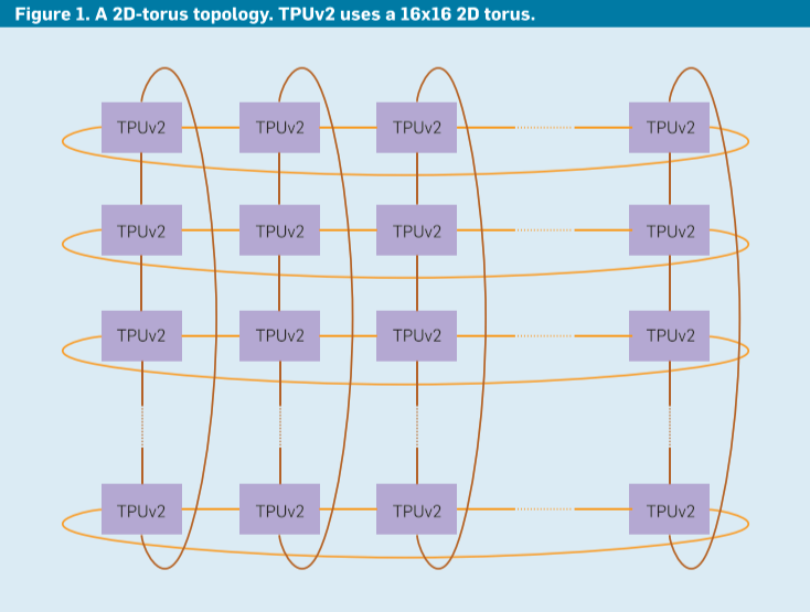
• what is the interconnect topology;
• does it have centralized versus distributed switches.

This choice is much easier for a DSA supercomputer, as the communication patterns are limited and known. For training, most traffic is an all-reduce over weight updates from all nodes of the machine.

If we distribute switch functionality into each chip rather than as a standalone unit, the all-reduction can be built in a dimension-balanced, bandwidth-optimal way for a 2D torus topology. An on-device switch provides virtual-circuit, deadlock-free routing. To enable a 2D torus, the chip has four custom Inter-Core Interconnect (ICI) links.

Designing a DSA supercomputer node

The TPUv2 node of the supercomputer followed the main ideas of TPUv1:

• A large two-dimensional matrix multiply unit (MXU) using a systolic array to reduce area and energy plus large;
• software-controlled on-chip memories instead of caches.

The large MXUs of the TPUs rely on large batch sizes, which amortize memory accesses for weights

Three regions for increasing batch size on training time

1. Perfect scaling region: Each doubling of batch size halves the number of training steps.
2. Diminishing returns region: Increasing batch size still reduces the number of steps, but more slowly.
3. Maximum data parallelism region: Increasing batch size provides no benefits whatsoever.

Unlike TPUv1, TPUv2 uses two cores per chip. Given that training can use many processors, two smaller TensorCores per chip prevented the excessive latencies of a single large full-chip core.

Six major blocks of a TensorCore

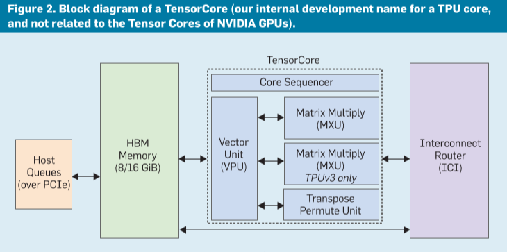
1. Inter-Core Interconnect (ICI). ICI enables direct connections between chips to form a supercomputer.
2. High Bandwidth Memory (HBM). TPUv1 was memory bound for most of its applications. We solved its memory bottleneck by using High Bandwidth Memory (HBM) DRAM in TPUv2. It offers 20 times the bandwidth of TPUv1 by using an interposer substrate that connects the TPUv2 chip via thirty-two 128-bit buses to four short stacks of DRAM chips.
3. The Core Sequencer fetches VLIW (Very Long Instruction Word) instructions from the core’s on-chip, software-managed Instruction Memory, executes scalar operations and forwards vector instructions to the VPU. The 322-bit VLIW instruction can launch eight operations: two scalar, two vector ALU, vector load and store, and a pair of slots that queue data to and from the matrix multiply and transpose units. (controlled by the XLA compiler) (instruction level parallel)
4. The Vector Processing Unit (VPU) performs vector operations using a large on-chip vector memory. The VPU collects and distributes data to Vmem via data-level parallelism (2D matrix and vector functional units) and instruction-level parallelism (8 operations per instruction).
5. The MXU produces 32-bit FP products from 16-bit FP inputs that accumulate in 32 bits.
   • The bandwidth required to feed and obtain results from an MXU is proportional to its perimeter, while the computation it provides is proportional to its area. Larger arrays provide more compute per byte of interface bandwidth, but larger arrays can be inefficient.
   • The reason is that some convolutions are naturally smaller than 256x256, so sections of the MXU would be idle. Sixteen 64x64 MXUs would have a little higher utilization (38%–52%) but would need more area.
   • The reason is the MXU area is determined either by the logic for the multipliers or by the wires on its perimeter for the inputs, outputs, and control. In our technology, for 128x128 and larger the MXU’s area is limited by the multipliers but area for 64x64 and smaller MXUs is limited by the I/O and control wires.
6. The Transpose Reduction Permute Unit does 128x128 matrix transposes, reductions, and permutations of the VPU lanes.

Alternative DSA supercomputer node design

TPUv3 has ≈1.35x the clock rate, ICI bandwidth, and memory bandwidth plus twice the number of MXUs, so peak performance rises 2.7x. Liquid cools the chip to allow 1.6x more power.

Designing DSA supercomputer arithmetic

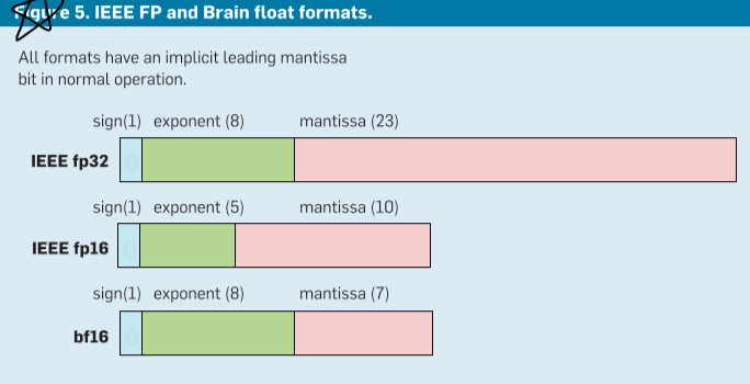
The resulting of brain floating format:

• Matrix multiplication outputs and internal sums must remain in fp32.
• The 5-bit exponent of fp16 matrix multiplication inputs leads to failure of computations that go outside its narrow range, which the 8-bit exponent of fp32 avoids.
• Reducing the matrix multiplication input mantissa size from fp32’s 23 bits to 7 bits did not hurt accuracy.

Designing a DSA Supercomputer Compiler

Introduction of XLA

TPUv2/v3s also use TF, with the new system XLA (for accelerated linear algebra) handling the TPU-dependent mapping. XLA also targets CPUs and GPUs.

XLA integrates a high-level library and a compiler. A TF front end generates code in an intermediate representation for XLA. (front ends + IR + back ends (CPU, GPU, TPU) )

Mapping at different levels

Beyond the parallelism of operations (“ops”) in a graph, each op can comprise millions of multiplications and additions on data tensors of millions of elements. XLA maps:

• the abundant parallelism across hundreds of chips in a supercomputer;
• a few cores per chip;
• multiple units per core;
• thousands of multipliers and adders inside each functional unit.

Standard VLIW compilation techniques

TPUs use a VLIW architecture to express instruction-level parallelism to the many compute units of a TensorCore.

XLA uses standard VLIW compilation techniques including loop unrolling, instruction scheduling, and software pipelining to keep all compute units busy and to simultaneously move data through the memory hierarchy to feed them.

Given a memory layout of data, operator fusion can reduce memory use and boost performance. Fusion is a traditional compiler optimization—but applied now to 2D data—that combines ops to reduce memory traffic compared to executing operators sequentially.

Contrasting GPU and TPU Architectures

Multi-chip parallelization is built into TPUs through ICI and supported through all-reduce operations plumbed through XLA to TF. Similarsized multi-chip GPU systems use a tiered networking approach, with NVIDIA’s NVLink inside a chassis and host-controlled InfiniBand networks and switches to tie multiple chassis together.

TPUs offer bf16 FP arithmetic designed for DNNs inside 128x128 systolic arrays; Volta GPUs have also embraced reduced-precision systolic arrays, with a finer granularity—4x4 or 16x16 depending on hardware or software descriptions—while using fp16 rather than bf16.

TPUs are dual-core, in-order machines, where the XLA compiler overlaps computation, memory, and network activities. GPUs are latency-tolerant manycore machines, where each core has many threads and thus very large (20MiB) register files.

TPUs use software controlled 32MiB scratchpad memories that the compiler schedules, while Volta hardware manages a 6MiB cache and software manages a 7.5MiB scratchpad memory. The XLA compiler directs sequential DRAM accesses typical of DNNs via direct memory access (DMA) controllers on TPUs while GPUs use multithreading plus coalescing hardware for them.

Background Knowledge

The contains of a layer

A layer contains a linear algebra part (often a matrix multiplication or convolution using the weights) followed by a nonlinear activation function (often a scalar function, applied elementwise; we call the results activations).

Embeddings as input data

Embeddings involve table lookups, link traversal, and variable length data fields.

Stochastic Gradient Descent (SGD)

How do we get from random initial weights to trained weights? Current best practices use variants of stochastic gradient descent (SGD). SGD consists of many iterations of three steps:

1. forward propagation;
2. backpropagation;
3. weight update.

Extensive Reading

• Asanovic´, K. Programmable neurocomputing. The Handbook of Brain Theory and Neural Networks, 2nd Edition. M.A. Arbib, ed. MIT Press, 2002.
• Hennessy, J.L. and Patterson, D.A. A new golden age for computer architecture. Commun. ACM 62, 2 (Feb. 2019), 48–60.
• Nicol, C. A dataflow processing chip for training deep neural networks. In Proceedings of the IEEE Hot Chips 29 Symp., (Aug 2017I.
• Shallue, C.J. et al. Measuring the effects of data parallelism on neural network training. 2018; arXiv preprint arXiv:1811.03600.