[Weekly Review] 2020/04/13-19

Published: April 19, 2020 by SingularityKChen (Last updated: April 19, 2020 )

• Categories:
• WeeklyReview 81

• Tags:
• CS61B 4
• Chisel 22
• Emulation 1
• Folding 1
• Formal 7
• Simulator 1
• Unfolding 1
• VCD 1

• 2020/04/13-19
  • CS61B
    • Binary Search Tree
    • B Trees
    • Rotation
    • Red-Black Trees
    • Hashing
    • Heap
    • Search Data Structures Summary (The particularly abstract ones)
    • Tree Traversals
    • Range Finding
  • Folding and Unfolding
    • Folding
    • Unfolding
  • Chisel Syntax
    • Dump VCDs in Chisel-Testers2
  • Get Ready For Verification 3.0
    • Continuum of verification engines
    • Verification 3.0

2020/04/13-19

CS61B

Binary Search Tree

A tree consists of:

• A set of nodes.
• A set of edges that connect those nodes.
  • Constraint: There is exactly one path between any two nodes.

A binary search tree is a rooted binary tree with the BST property.

BST Property. For every node X in the tree:

• Every key in the left subtree is less than X’s key.
• Every key in the right subtree is greater than X’s key.

runtime to complete a search on a “bushy” BST in the worst case is Θ(log N) and the height of the tree is ~log2(N).

Deleting

• Key with no Children: Just sever the parent’s link
• Key with one Child: Move it’s parent’s pointer to it’s child.
• Key with two Children:
  • Find a new root node.
  • Must be > than everything in left subtree.
  • Must be < than everything right subtree.

Tree Height

Height varies dramatically between “bushy” and “spindly” trees.

H = Θ(log(N))

H = Θ(N)

BSTs have potential performance issue if they get “spindly”

B Trees

A B-tree of order M=4 is also called a 2-3-4 tree or a 2-4 tree.

The name refers to the number of children that a node can have, e.g. a 2-3-4 tree node may have 2, 3, or 4 children.

B-Trees are most popular in two specific contexts:

• Small M (M=3 or M=4):
  • Used as a conceptually simple balanced search tree (as today).
• M is very large (say thousands)
  • Used in practice for databases and filesystems (i.e. systems with very large records).

Note: Since the small M tree isn’t practically useful (as we’ll see in a few slides, people usually only use the name B-tree to refer to the very large M case.

• If we split the root, every node gets pushed down by exactly one level.
• If we split a leaf node or internal node, the height doesn’t change.

Rotation

Rotation: Can shorten (or lengthen) a tree or preserves search tree property.

Red-Black Trees

Goal: Represent a 2-3 Tree as a Binary Tree

LLRBs mimic 2-3 tree behavior using color flipping (and tree rotation).

• Height is guaranteed logarithmic.
• After insert/delete, at most 1 color flip or rotation per level of the tree.
  • Since height is logarithmic, we have O(log N) flips/rotations.
  • insert/delete operations are therefore O(log N).
• Easier to implement, constant factor faster than 2-3 or 2-3-4 tree.

Hashing

DataIndexedIntegerSet Implementation

public class DataIndexedIntegerSet {
	boolean[] present;
 
	public DataIndexedIntegerSet() {
    	present = new boolean[16];
	}
 
	public insert(int i) {
    	present[i] = true;
	}
 
	public contains(int i) {
    	return present[i];
	}
}

Θ(1)

External Chaining

• If we use the 10 buckets on the right, where should our six items go?
  • Put in bucket = hash Code % 10
• If N items are distributed across M buckets, average time grows with N/M = L, also known as the load factor.
  • Average runtime is Θ(L).

	contains(x)	insert(x)
Linked List	Θ(N)	Θ(N)
Bushy BSTs	Θ(log N)	Θ(log N)
Unordered Array	Θ(N)	Θ(N)
Hash Table	Θ(1)	Θ(1)

With good hashCode() and resizing, operations are Θ(1) amortized.

Heap

Binary min-heap: Tree that is complete and obeys min-heap property. Can be used for the priority queue.

• Min-heap: Every node is less than or equal to both of its children.
• Complete: Missing items only at the bottom level (if any), all nodes are as far left as possible.

Search Data Structures Summary (The particularly abstract ones)

Name	Storage Operation	Primary Retrieval Operation	Retrieve By:
List	add(key), insert(key, index)	get(index)	index
Map	put(key, value)	get(key)	key identity
Set	add(key)	containsKey(key)	key identity
PQ	add(key)	getSmallest()	key order (a.k.a. key size)
Disjoint Sets	connect(int1, int2)	isConnected(int1, int2)	two int values

Tree Traversals

Tree traversal, or tree iteration.

Depth First Traversals

Preorder traversal: “Visit” a node, then traverse its children: DBACFEG

Inorder traversal: Traverse left child, visit, then traverse right child: ABCDEFG

Postorder traversal: Traverse left, traverse right, then visit: ACBEGFD

Range Finding

Pruning: Restricting our search to only nodes that might contain the answers we seek.

Runtime for find-In-Range search: Θ(log N + R)

• N: Total number of items in tree.
• R: Number of matches.

Spatial (a.k.a. Geometric) Trees

Handling Multidimensional Data: Quadtrees

Quadtrees: Divide and conquer by splitting 2D space into four quadrants.

• Store items into appropriate quadrant.
• Repeat recursively if more than one item in a quadrant.

Folding and Unfolding

Folding

Folding is Time-Shared Architecture

• Folding is a technique to reduce the silicon area by time multiplexing many operations into single function units
• Folding introduces registers
• Computation time increased

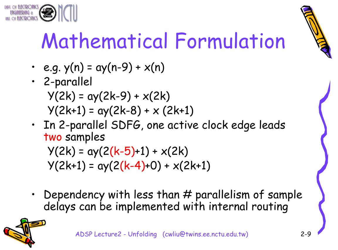
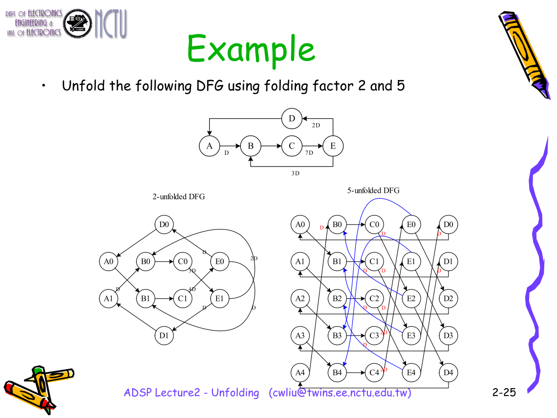
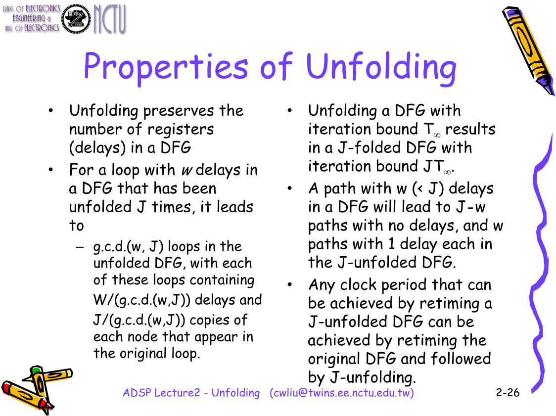
Unfolding

Unfolding is the process of unfolding a loop so that several iterations are unrolled into the same iteration.

• Also known as (a.k.a.)
  • Loop unrolling (in compilers for parallel programs)
  • Block processing
• Applications – Reducing sampling period to achieve iteration bound (desired throughput rate) T∞.
  • Parallel (block processing) to execute several iterations concurrently.
  • Digit-serial or bit-serial processing

Chisel Syntax

Dump VCDs in Chisel-Testers2

I found three methords to dump VCDs in chisel testers2. The first two are more friendly for people who develop the project with Intellij Idea, as you can simply click the run bottom and then can get both the simulation results and the VCD file.

Test.withAnnotations

If you want to get the waveform of your testbench with chisel tetsers2, you can add WriteVcdAnnotation argument to test with the help of withAnnotations. To use the arguments, you neeed import WriteVcdAnnotation and WriteVcdAnnotation. Here is an example.

import chisel3.tester._
import chisel3.tester.experimental.TestOptionBuilder._
import chiseltest.internal.WriteVcdAnnotation
import org.scalatest._

class ClusterGroupSpecTest extends FlatSpec with ChiselScalatestTester with Matchers {
  behavior of "XXXX"
  it should "XXXX" in {
    test (new Module)).withAnnotations(Seq(WriteVcdAnnotation)) { dut => 
    }
  }
}

RawTester

Also, you can use RawTester and add some arguments at the same time, which including WriteVcdAnnotation.

import chiseltest._
import chiseltest.internal.WriteVcdAnnotation

RawTester.test(module, Seq(WriteVcdAnnotation)) { dut =>
}

Add arguments in Shell

Maybe you can also run the test with runtime arguments in sbt shell.

$bash: sbt
sbt > testOnly chiseltest.tests.BasicTest -- -DwriteVcd=1

Get Ready For Verification 3.0

Continuum of verification engines

Verification 1.0 was dominated by the simulator running on individual workstations. Verification 2.0 added emulation and formal verification as mainstream technologies, making use of simulation farms.

Simulator

A simulator is a piece of software that exercises a model of hardware. It can be written using several levels of abstraction and use a variety of languages. Such as SPICE, Verilog or VHDL languages and SystemC.

Assuming you have a model, the simulator will exercise that model and observe its behaviors based on the stimulus that is supplied to it. For an act of verification, you need to ensure that the design behaves as intended.

The collection of stimulus, checkers, coverage, constraints and result predictor is called a testbench.

Emulation

Emulation is a technology whereby the design is transformed into an implementation capable of being executed on special purpose hardware. This implementation has no correspondence with the final implementation which would target a particular technology library.

Instead, an emulator has a number of blocks capable of taking on a function (such as an FPGA), a programmable interconnect (although some early emulators used fixed interconnect) and a software tool chain that attempts to divide the circuit amongst the programmable elements, configure the interconnect and provide a runtime environment that makes the emulator look similar to a logic simulator.

An emulator can either be connected to a testbench or other part of the circuit running in a logic simulator. This is sometimes called co-emulation or simulation acceleration. Alternatively, the emulator can be connected to a live system. This is usually called in-circuit emulation.

Formal Verification

Equivalence checking

This takes two designs, that may be at the same or different levels of abstraction and finds functional differences between them.

Combinatorial equivalence checking (logic functions)

Combinatorial equivalence checking is used to show that a design after logic synthesis is the same as the input RTL description. It is also used to show that no functionality has been affected when test logic or other gate-level transformations are made. It compares the combinatorial logic between corresponding registers in the original description.

Sequential equivalence checking (design qualities)

Sequential equivalence checking is an emerging technology that can take two designs that have fundamentally different timing, enabling an un-timed or partially timed model to be compared against an RTL model, or between RTL models that have undergone retiming or other transformation to improve power or other design qualities. This is a necessary technology for mass adoption of high-level synthesis.

Property checking

A property defines a behavior that must be present in a design, or a behavior that must not be possible. A third option is called a fairness condition that would ensure that each of several options is not treated unfairly, in arbitration for example.

Verification 3.0

Up until Verification 3.0, the only thing that most teams had to worry about was functionality. Today, that is often the easy part of what the verification team is tasked with. Teams are taking on additional roles in power verification, performance verification and, increasingly, safety and security requirements.

Portable Stimulus has a large role to play here. Verification at this level is not just about hardware execution (e.g. cache coherency), but also software functionality.