[Weekly Review] 2020/04/20-26

Published: April 26, 2020 by SingularityKChen (Last updated: April 26, 2020 )

• Categories:
• WeeklyReview 81

• Tags:
• Agile 3
• CLINT 1
• Graph 1
• JVM 1
• Models 1
• PLIC 1
• SystemC 15

• 2020/04/20-26
  • CS61B
    • Graph
  • Scheduling
    • ASAP & ALAP
  • Agile Hardware Development
  • Models and Abstractions
    • Temporal abstraction
    • Data abstraction
    • Functionality abstraction
    • Concurrency
    • Communications
    • Configurability
  • C++
  • SystemC
    • Books
  • JVM Memory
    • Heap and Non-Heap Memory
  • Rocket Chip
    • CLINT (Core Local Interrupter)
    • PLIC (Plantform Level Interrpt Controller)

2020/04/20-26

This week, I continued to debug the Eyeriss implementation and verification. Also, I began to write the final thesis and draw the architecture diagrams at the same time. Currently, I have finished the draft of six chapters of my thesis.

While I was debugging with waveform in gtkwave, I found that I could not obtain the whole waveform of cluster group test, as it was too large to be generated. Sequencer told me that might be memory leak leaded by JVM.

I also learned that SystemC can abstract two kinds of timing models: Loosely Timed (LT) and Approximately Timed (AP). The former is used for software execution while the later is used for architectural exploration.

CS61B

Graph

Graph: A set of nodes (a.k.a. vertices) connected pairwise by edges.

Graph Terminology

• Graph:
  • Set of vertices, a.k.a. nodes.
  • Set of edges: Pairs of vertices.
  • Vertices with an edge between are adjacent.
  • Optional: Vertices or edges may have labels (or weights).
• A path is a sequence of vertices connected by edges.
• A cycle is a path whose first and last vertices are the same.
  • A graph with a cycle is ‘cyclic’.
• Two vertices are connected if there is a path between them. If all vertices are connected, we say the graph is connected.

Graph Problem

s-t Path. Is there a path between vertices s and t?

Shortest s-t Path. What is the shortest path between vertices s and t?

Cycle. Does the graph contain any cycles?

Euler Tour. Is there a cycle that uses every edge exactly once?

Hamilton Tour. Is there a cycle that uses every vertex exactly once?

Connectivity. Is the graph connected, i.e. is there a path between all vertex pairs?

Biconnectivity. Is there a vertex whose removal disconnects the graph?

Planarity. Can you draw the graph on a piece of paper with no crossing edges?

Isomorphism. Are two graphs isomorphic (the same graph in disguise)?

Graph problems: Unobvious which are easy, hard, or computationally intractable.

Graph Representations

Representation 1: Adjacency Matrix

0 -> 1, 0- > 2, 1 -> 2.

s\t	0	1	2
0	0	1	1
1	0	0	1
2	0	0	0

Representation 2: Edge Sets: Collection of all edges

{(0, 1), (0, 2), (1, 2)}

Representation 3: Adjacency lists

table	->	value
0	->	[1,2]
1	->	[2]
2	->

idea	addEdge(s, t)	adj(s)	hasEdge(s, t)	space used
adjacency matrix	Θ(1)	Θ(V)	Θ(1)	Θ(V^2)
list of edges	Θ(1)	Θ(E)	Θ(E)	Θ(E)
adjacency list	Θ(1)	Θ(1)	Θ(degree(v))	Θ(E+V)

DepthFirstPaths: s-t Path

Properties of Depth First Search:

• Guaranteed to reach every node.
• Runs in O(V + E) time.
  • Analysis next time, but basic idea is that every edge is used at most once, and total number of vertex considerations is equal to number of edges.
  • Runtime may be faster for problems which quit early on some stopping condition (for example connectivity).
• Θ(V) space

Topological Sort

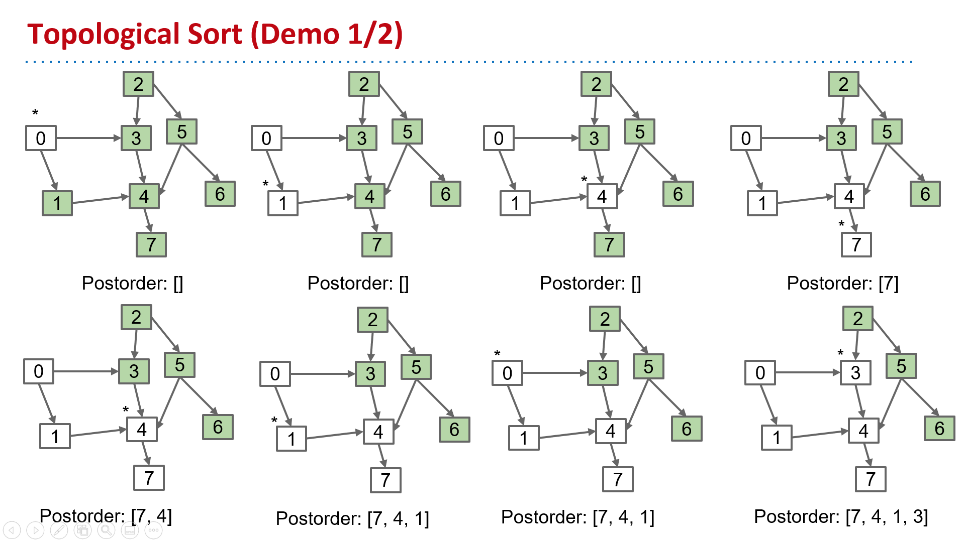
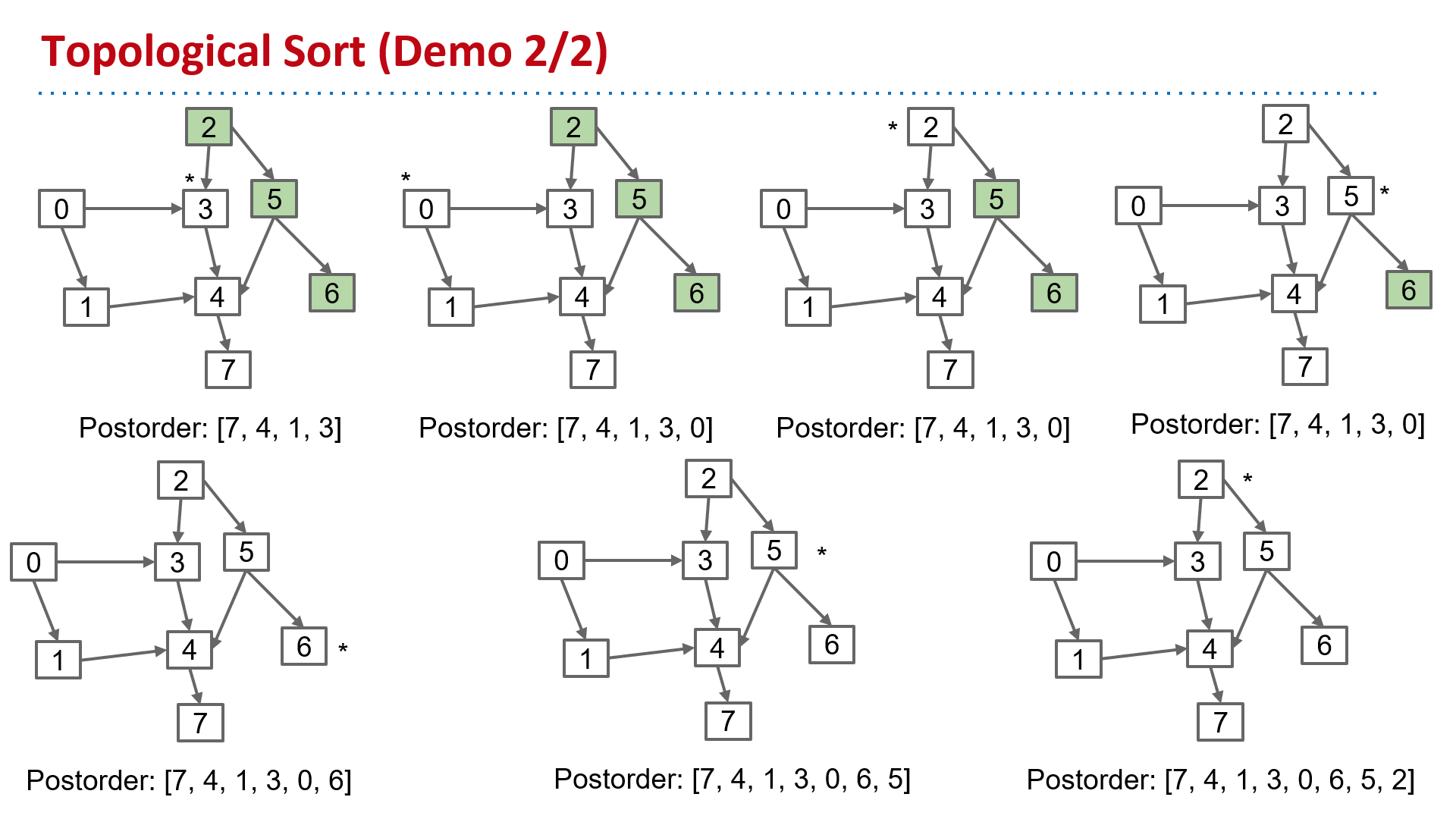
Find an ordering of vertices consistent with directed edges.

Θ(V+E) time, Θ(V) space

Breadth First Search: Shortest s-t Path (BFS)

• Initialize a queue with a starting vertex s and mark that vertex.
  • Let’s call this the fringe.
• Repeat until queue is empty:
  • Remove vertex v from queue.
  • Add to the queue any unmarked vertices adjacent to v and mark them.
• Runs in O(V + E) time.
• Θ(V) space.

Dijkstra’s Algorithm: Finding a Shortest Paths Tree

Visit vertices in order of best-known distance from source, relaxing each edge from the visited vertex (relax an edge: Add to SPT if better distance).

Priority Queue operation count, assuming binary heap based PQ:

• Insertions: V, each costing O(log V) time.
• Delete-min: V, each costing O(log V) time.
• decrease Priority: E, each costing O(log V) time.
  • Data structure not discussed in class.

Overall runtime: O(Vlog(V) + Vlog(V) + E*logV).

• Assuming E > V, this is just O(E log V).

Graph Problem Summary

Problem	Problem Description	Solution	Efficiency
paths	Find a path from s to every reachable vertex.	DepthFirstPaths.java Demo, Iterative Demo	Θ(V+E) time Θ(V) space
topological sort	Find an ordering of vertices consistent with directed edges.	DepthFirstOrder.java Demo	Θ(V+E) time Θ(V) space
shortest paths	Find the shortest path from s to every reachable vertex.	BreadthFirstPaths.java Demo	Θ(V+E) time Θ(V) space
shortest weighted paths	Find the shortest path, considering weights, from st to every reachable vertex.	DijkstrasSP.java Demo	Θ(E log V) time Θ(V) space

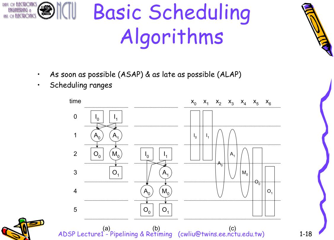
Scheduling

ASAP & ALAP

Agile Hardware Development

Agile hardware development is an approach whereby frameworks and practices normally associated with agile software are applied in the development of IP, FPGAs, ASICs and/or SoCs.

Agile software practitioners have found that success depends on treating product software development as more than an impersonal, pre-defined, assembly line process where individuals toss code from cubicle to cubicle.

These practices would include iterative development and continuous deployment among others. Likewise, even in ASIC and SoC development where target technology imposes serious restrictions on flexibility, teams may still find value in using various agile development practices such as iterative development, test-first programming, pair programming and continuous integration.

Models and Abstractions

A model is an abstraction of a device. Many models, such as those written in Verilog or VHDL, are executable. Being executable means that a tool, such as a simulator or emulator, can exercise the model and, when stimulated, produce results. Other models are not executable, but instead contain information that can be read by a tool, manipulated and written back. These models, such as a coverage model, may control a flow.

These can be at a number of abstractions including SPICE, transistor, RTL, or one of many ESL abstractions. Designs for SoC flows tend to be abstractions in the temporal axis, the data axis or the functionality axis. The introduction of ESL modeling has added three additional forms of abstraction, namely concurrency, communications and configurability.

Temporal abstraction

The temporal axis defines the timing in the model. Certain tasks within a design flow require sub-clock cycle accuracy and analog design usually has whatever timing accuracy is necessary in order to ensure all changes are piecewise linear.

Data abstraction

The data axis defines the level of precision of data. At the highest level, data may be abstracted to an event without any actual concept of the actual data. Within an ESL flow, it is typical to work with transactions which hold packets of data that have no correspondence with the way in which data would actually be organized in the final system.

Functionality abstraction

This attempts to define the precision of the operations themselves. For example, a mathematical formula defines precedence but not order. The algorithm must be scheduled and this is often the operation performed during high-level synthesis.

Concurrency

Concurrency defines the amount of processing or execution of an application that can be performed simultaneously. Concurrency is sometimes restricted by the model of computation imbedded in a language. For example, the C language is a sequential language and so a tool has to extract the available concurrency that may exist in the model by performing dependency analysis. Other languages allow for concurrency to be described directly.

Communications

When more than one processing element exists, there must be communications between them. That communication can take many forms and is highly dependent on the architecture of the final solution. Very fine grained parallelism such as operations within an instruction or dedicated pieces of hardware are naturally handled by point to point communication or pipelines. At the other end of the spectrum, two software threads that need to communicate are likely to use some form of shared-memory to communicate with one another.

Configurability

How fixed is the design? An ASIC generally embeds all aspects of the design in hardware and they cannot be modified, but in many cases, a certain degree of flexibility is built into devices.

A processor with a fixed instruction set is also considered a fixed solution. However, a processor with an extensible instruction set has some degree of configurability. This configurability is handled by the tools in the design path. Hardware can also be built to be configurable.

C++

The C and C++ language have an important role to play within the EDA industry. Not only are most EDA programs developed in these languages, but they are also the most popular language used for the creation of virtual prototypes. Virtual prototypes are functional models of an electronic system and are often used to study the high-level behavior of systems under development so that aspects such as system functionality and performance can be assessed.

In 1996, the EDA industry started work creating a class library built on top of C++ that added notion of hardware concurrency, timing and supporting the extended value set seen in hardware. This was first released in 2000 and became know as SystemC. It is the primary language used as input to high-level synthesis tools.

SystemC

SystemC is a class library built on top of the C++ language.

The class library, together with a set of macros, implements an event-driven simulator. The principle extensions beyond C++ are the ability to define concurrency, to add timing information and an extended set of datatypes.

Version 1.0 of the standard, released Mar 28th 2000, mimicked the existing Hardware Description Languages (HDL) in that it provided a structural hierarchy, signal-level connectivity, clock-cycle accuracy, delta cycles necessary for dealing with zero delays, four-valued logic (0, 1, X, Z), and bus-resolution functions. A reference implementation was provided as the standard.

Version 2, released Feb 1st 2001, extended SystemC into a higher level of abstraction adding abstract communications, transaction-level modeling, and capabilities for the creation of virtual platforms (VP) modeling. This release added abstract ports, dynamic processes, and timed event notifications.

Given that is was possible to define multiple levels of abstraction with 2.0, two sets of recommended abstractions were defined called Loosely Timed (LT) and Approximately Timed (AP). LT models had minimal timing defined. These would be fast executing models aimed at virtual prototypes developed for software execution. AP models had a lot more timing information included and would be better suited for performance analysis, architectural exploration and form the basis of a hardware development flow.

Books

Transaction Level Modeling with SystemC: TLM Concepts and Applications for Embedded Systems

SystemC: From the Ground Up

SystemC and SystemC-AMS in Practice: SystemC 2.3, 2.2 and SystemC-AMS 1.0

Complete Symbolic Simulation of SystemC Models: Efficient Formal Verification of Finite Non-Terminating Programs

JVM Memory

The JVM is an abstract computing machine that enables a computer to run a Java program.

The JVM loads the code, verifies the code, executes the code, manages memory (this includes allocating memory from the Operating System (OS), managing Java allocation including heap compaction and removal of garbage objects) and finally provides the runtime environment.

Heap and Non-Heap Memory

The JVM memory consists of the following segments:

• Heap Memory, which is the storage for Java objects
• Non-Heap Memory, which is used by Java to store loaded classes and other meta-data
• JVM code itself, JVM internal structures, loaded profiler agent code and data, etc.

Heap

The JVM has a heap that is the runtime data area from which memory for all class instances and arrays are allocated. It is created at the JVM start-up.

The heap size may be configured with the following VM options:

• -Xmx<size> - to set the maximum Java heap size

• -Xms<size> - to set the initial Java heap size

  By default, the maximum heap size is 64 Mb.

Non-Heap

Also, the JVM has memory other than the heap, referred to as non-heap memory. It is created at the JVM startup and stores per-class structures such as runtime constant pool, field and method data, and the code for methods and constructors, as well as interned Strings.

If the application indeed needs that much of non-heap memory and the default maximum size of 64 Mb is not enough, you may enlarge the maximum size with the help of -XX:MaxPermSize VM option. For example, -XX:MaxPermSize=128m sets the size of 128 Mb.

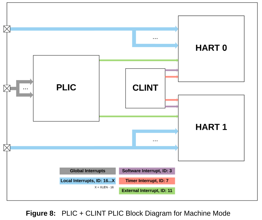
Rocket Chip

CLINT (Core Local Interrupter)

The CLINT has a fixed priority scheme which implements Software, Timer, and External interrupts. Software preemption is only available between privilege levels using the CLINT. For example, while in Supervisor mode, a Machine mode interrupt will immediately take priority and preempt Supervisor mode operation. Preemption within a privilege level is not supported with the CLINT. The interrupt ID represents the fixed priority value of each interrupt, and is not configurable. There are two different CLINT modes of operation, direct mode and vectored mode.

To configure CLINT modes, write mtvec.mode field, which is bit[0] of mtvec CSR. For direct mode, mtvec.mode=0, and for vectored mode mtvec.mode=1.

Direct mode is the default reset value. The mtvec.base holds the base address for interrupts and exceptions, and must be a minimum 4-byte aligned value in direct mode, and minimum 64-byte aligned value in vectored mode.

PLIC (Plantform Level Interrpt Controller)

The PLIC is used to manage all global interrupts and route them to one or many CPUs in the system. It is possible for the PLIC to route a single interrupt source to multiple CPUs. Upon entry to the PLIC handler, a CPU reads the claim register to acquire the interrupt ID. A successful claim will atomically clear the pending bit in the PLIC interrupt pending register, signaling to the system that the interrupt is being serviced.

During the PLIC interrupt handling process, the pending flag at the interrupt source should also be cleared, if necessary. It is legal for a CPU to attempt to claim an interrupt even when the pending bit is not set. This may happen, for example, when a global interrupt is routed to multiple CPUs, and one CPU has already claimed the interrupt just prior to the claim attempt on another CPU.

Before exiting the PLIC handler with MRET instruction (or SRET/URET), the claim/complete register is written back with the non zero claim/complete value obtained upon handler entry. Interrupts routed through the PLIC incur an additional three cycle penalty compared to local interrupts. Cycles in this case are measured at the PLIC frequency, which is typically an integer divided value from the CPU and local interrupt controller frequency.