[Weekly Review] 2020/04/27-05/03
Published:
by
SingularityKChen
![]() (Last updated:
)
(Last updated:
)
- Categories:
- WeeklyReview 81
2020/04/27-05/03
This week I stopped learning CS61B and to modelling Eyeriss and CPU processing MAC. And I also focused on my thesis, which was almost finished the draft version.
Unfortunately, the TEP visa and airline ticket affected my efficiency this week.
I'll continue to polish my thesis and FYP until next Wednesday, then I'll turn to prepare for the GRE test or TPT test.
CS61B
A*
Dijkstra’s problem: will explore every place within nearly two thousand miles of Denver before it locates NYC.
Simple idea:
- Visit vertices in order of d(Denver, v) + h(v), where h(v) is an estimate of the distance from v to NYC.
- In other words, look at some location v if:
- We know already know the fastest way to reach v.
- AND we suspect that v is also the fastest way to NYC taking into account the time to get to v.
Spanning Tree
Given an undirected graph, a spanning tree T is a subgraph of G, where T:
- Is connected. -> tree
- Is acyclic. -> tree
- Includes all of the vertices -> spanning
Prim’s Algorithm
Start from some arbitrary start node.
- Repeatedly add shortest edge (mark black) that has one node inside the MST under construction.
- Repeat until V-1 edges.
Prim’s and Dijkstra’s algorithms are exactly the same, except for the following:
- Visit order:
- Dijkstra’s algorithm visits vertices in order of distance from the source.
- Prim’s algorithm visits vertices in order of distance from the MST under construction.
- Visitation:
- Visiting a vertex in Dijkstra’s algorithm means to relax all of its edges.
- Visiting a vertex in Prim’s algorithm means relaxing all of its edges, but under the metric of distance from tree instead of distance from source.
| Operation | Number of Times | Time per Operation | Total Time |
|---|---|---|---|
| Insert | V | O(log V) | O(V log V) |
| Delete minimum | V | O(log V) | O(V log V) |
| Decrease priority | E | O(log V) | O(E log V) |
Kruskal’s Algorithm
Initially mark all edges gray.
- Consider edges in increasing order of weight.
- Add edge to MST (mark black) unless doing so creates a cycle.
- Repeat until V-1 edges.
| Operation | Number of Times | Time per Operation | Total Time |
|---|---|---|---|
| Build-PQ of edges | 1 | O(E) | O(E) |
| Delete minimum | E | O(log E) | O(E log E) |
| connect | V | O(log* V) | O(V log* V) |
| isConnected | E | O(log* V) | O(E log*V) |
Shortest Paths and MST Algorithms Summary
| Problem | Algorithm | Runtime (if E > V) | Notes |
|---|---|---|---|
| Shortest Paths | Dijkstra’s | O(E log V) | Fails for negative weight edges. |
| MST | Prim’s | O(E log V) | Analogous to Dijkstra’s |
| MST | Kruskal’s | O(E log E) | Uses WQUPC |
| MST | Kruskal’s with pre-sorted edges | O(E log* V) | Uses WQUPC |
Dynamic Programming
The DAG SPT algorithm can be thought of as solving increasingly large subproblems:
- Distance from source to source is very easy, and is just zero.
- We then tackle distances to vertices that are a bit farther to the right.
- We repeat this until we get all the way to the end of the graph.
Problems grow larger and larger.
- By “large” we informally mean depending on more and more of the earlier subproblems.
This approach of solving increasingly large subproblems is sometimes called dynamic programming.
Dynamic programming is a terrible name for a simple and powerful idea for solving “big problems”:
- Identify a collection of subproblems.
- Solve subproblems one by one, working from smallest to largest.
- Use the answers to the smaller problems to help solve the larger ones.
Longest Increase Subsequence(LIS)
Given a sequence of integers, we transformed our problem into a problem on DAGs.
- This process is sometimes called reduction.
- We “reduced” LLIS to N solutions of the longest paths problem on DAGs.
Approach 1: Reduce LLIS to N executions of DAGSPT. Runtime was Θ(N3)
Approach 2A: Define subproblems Q[0] through Q[N - 1]. Runtime is Θ(N2)
- Can use DAG + solutions to Q[0] through Q[K-1] to solve Q[K]
- LLIS solution is max of all Q values.
Approach 2B: Define subproblems Q[0] through Q[N - 1]. Runtime is Θ(N2)
- Can use array + solutions to Q[0] through Q[K-1] to solve Q[K]
- LLIS solution is max of all Q values.
High Speed Cache
Cache Basic
How the cache affect coding
Two different code:
int arr[10][128];

for (i = 0; i < 10; i++)
        for (j = 0; j < 128; j++);
                arr[i][j] = 1;

int arr[10][128];

for (i = 0; i < 128; i++)
        for (j = 0; j < 10; j++);
                arr[j][i] = 1;
The processing of read/write data from/into main memory:
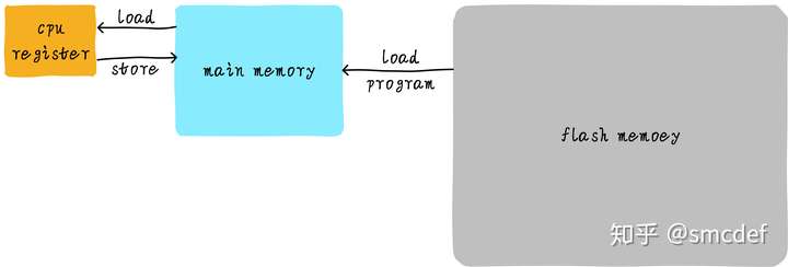
But the operation on main memory is too low, so we can add a cache between CPU registers and main memory. Hence the code bellow becomes the operation between CPU registers and the cache.

However, the size of cache is limited, and if cache miss, then cache will load from main memory. If we write code in the former style, then we will hit for a major time. If we use the second styles, then the cache will always miss if the cache is smaller than one row.
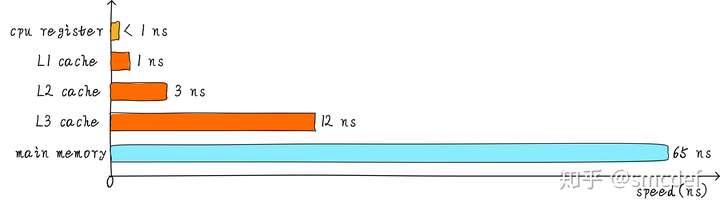
Hierarchy cache
To meet the requirements between storage and operate speed.
Cooperate between hierarchy cache
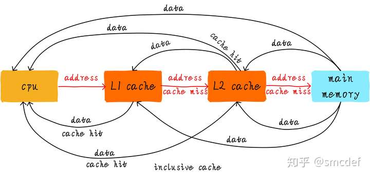
Inclusive cache means one address's value can exists in different level's cache. Exclusive cache means it only exists on one cache.
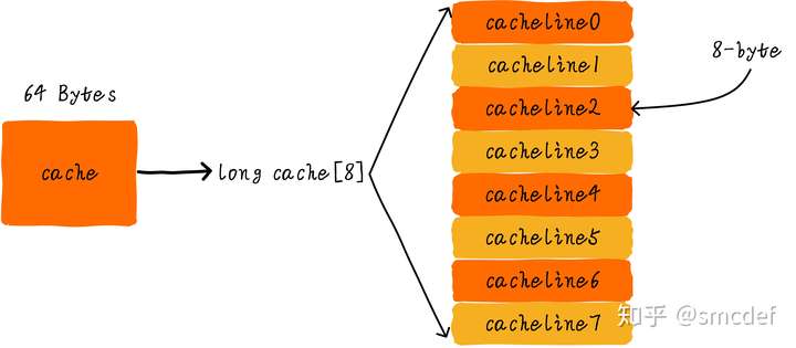
Cache line
cache size = cache line * cache line size
Cache line is the smallest transferring size between main memory. For instance, if CPU want to read one bit of cache miss data, then the cache have to read one cache line size of data from main memory.
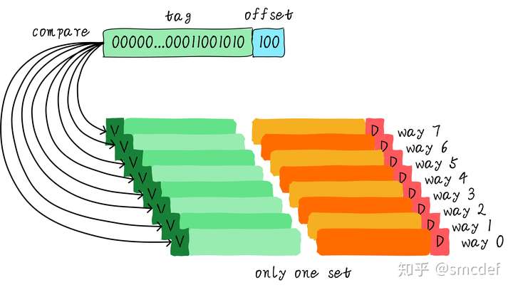
Cache offset, tag
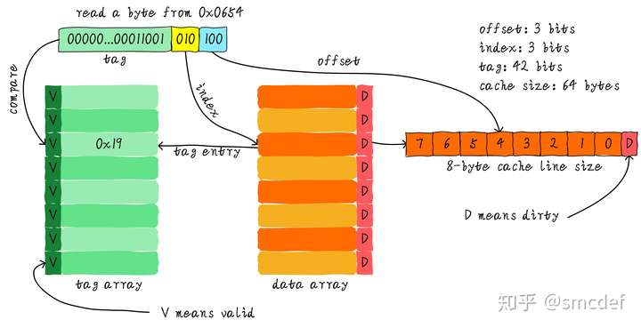
We use index to lookup one cache line, use offset to lookup the data in the cache line. Then the other bits of address are tag.
If we want to see whether one address is in the cache, then firstly read the index, then read and compare the corresponding tag. If equals and valid is true, then can read the value with offset.
Direct mapped cache
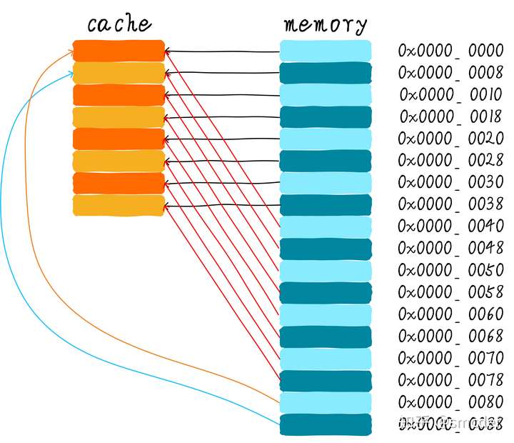
Cache thrashing
For instance, if we want to read 0x00, 0x40, 0x80, and both index and offset are 3-bits, then these three addresses' index are same, equal to zero. Then the first time it reads 0x00 from main memory into cache line zero. The second time it reads 0x40 and write into cache line zero too. That's cache thrashing.
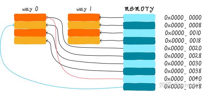
Two-way associative cache
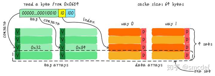
One set contains all the ways that have the same cache line index.
Then if need read, then read all the tags according to the index, and compare all the tags. The cache can hit while one tag equals to the one we need to read.
Full associative cache
Cache allocation policy
Read allocation
While CPU read cache miss, then will have one cache line to store the new data from memory.
Write allocation
If CPU want to write but cache miss, then it can write directly back to main memory. Or it can firstly read the corresponding memory, then write it to the cache line.
Cache update policy
Write through
Update the data in the cache line and main memory.
Write back
Use one dirty bit to show this cache line's data has been written and can not be overwritten by the data from main memory. So it has to write back to main memory if this cache line is going to be overwritten.